Mean-Variance Portfolio

Portfolio optimization involves the strategic allocation of wealth across various assets, including stocks, bonds, commodities, and other investment instruments. The objective of portfolio optimization is to construct portfolios that strike an optimal balance between expected returns and risk.

To achieve this, portfolio optimization can take into consideration several factors, including historical data, market trends, and the investor’s risk tolerance. Expected returns and variances play a crucial role in the process. Expected returns estimate the potential gains an investor anticipates from holding a particular asset, while variances measure the volatility or fluctuation in the assets’ returns.

The efficient frontier is a key concept in portfolio optimization. It represents the set of portfolios that offer the highest expected returns for a given level of risk. This Mod returns portfolios on the efficient frontier given expected returns and variances.

Problem Specification

We consider a single-period portfolio optimization problem where want to allocate wealth into \(n\) risky assets. The returned portfolio \(x\) is an efficient mean-variance portfolio for given returns \(\mu\), covariance matrix \(\Sigma\) and risk aversion \(\gamma\).

Background: Mathematical Formulation

The most basic version of this Mod is implemented by formulating a Quadratic Program (QP) and solving it using Gurobi. The formulation is as follows:

\[\begin{split}\begin{alignat}{2} \max \quad & \mu^\top x - \tfrac12 \gamma\ x^\top\Sigma x \\ \mbox{s.t.} \quad & 1^\top x = 1 \\ \end{alignat}\end{split}\]

• \(\mu\) is the vector of expected returns.

• \(\Sigma\) is the return covariance matrix.

• \(x\) is the portfolio where \(x_i\) denotes the fraction of

  wealth invested in the risky asset \(i\).

• \(\gamma\geq0\) is the risk aversion coefficient.

This description refers only to the simple base model. Further down in Enforcing more portfolio features we explain how to enforce additional features, such as leverage or transaction fees.

Data Specification

The mean-variance portfolio optimization model takes the following inputs:

• The covariance matrix \(\Sigma\) can be given as a pandas DataFrame or a numpy array.

• The return estimator \(\mu\) can be given as a pandas Series or a numpy array.

The returned allocation vector \(x\) is a pandas Series or a numpy ndarray (depending on the input types).

Example

Here we derive the matrix \(\Sigma\) and the vector \(\mu\) from a time series of historic excess returns:

>>> from gurobi_optimods import datasets
>>> data = datasets.load_portfolio()
>>> data
            AA        BB        CC  ...        HH        II        JJ
0   -0.000601  0.002353 -0.075234  ...  0.060737 -0.012869 -0.022137
1    0.019177  0.050008  0.041345  ... -0.026674  0.009876  0.012809
2   -0.020333  0.026638 -0.038999  ... -0.023153 -0.007007 -0.038034
3    0.001421 -0.053813 -0.013347  ... -0.012348  0.018736 -0.058373
4    0.008648  0.114836  0.003617  ...  0.064090 -0.011153  0.024333
..        ...       ...       ...  ...       ...       ...       ...
240  0.007382 -0.000724 -0.002444  ... -0.007654  0.018015 -0.017135
241 -0.003362 -0.106913 -0.082365  ...  0.040787 -0.023020 -0.067792
242  0.004359 -0.029763 -0.041986  ...  0.014522 -0.017109 -0.060247
243 -0.018402 -0.054211 -0.075788  ... -0.013557  0.022576 -0.036793
244 -0.016237  0.015580 -0.026970  ... -0.005893 -0.013456 -0.032203

[245 rows x 10 columns]

The columns of this DataFrame represent the individual assets (“AA”, “BB”, …, “JJ”) while the rows represent the historic time steps. We use pandas functionality to compute a simple mean estimator and corresponding covariance from this DataFrame:

import pandas as pd

from gurobi_optimods.datasets import load_portfolio
from gurobi_optimods.portfolio import MeanVariancePortfolio

data = load_portfolio()
cov_matrix = data.cov()
mu = data.mean()
gamma = 100.0

mvp = MeanVariancePortfolio(mu, cov_matrix)
pf = mvp.efficient_portfolio(gamma)

Solution

The method efficient_portfolio returns a PortfolioResult instance, containing information on the computed portfolio. It has the following attributes:

• x : The relative investments \(x\) for each asset

• ret : The estimated return \(\mu^T x\)

• risk : The estimated risk \(x^T \Sigma x\)

In this example the solution suggests to spread the investments over five positions (AA, DD, GG, HH, II). The other allocations are negligible.

>>> pf.x
AA    4.236507e-01
BB    1.743570e-07
CC    7.573610e-10
DD    2.430104e-01
EE    1.017732e-07
FF    2.760531e-09
GG    2.937307e-02
HH    2.350833e-01
II    6.888222e-02
JJ    1.248442e-08
dtype: float64

The estimated risk and return are:

>>> round(pf.risk, ndigits=8)
0.00017552
>>> round(pf.ret, ndigits=8)
0.00365177

Using factor models as input

In the preceding discussion we have assumed that we the covariance matrix \(\Sigma\) was explicitly given. In many cases, however, the covariance is naturally given through a factor model. Mathematically, this means that a decomposition

\[\begin{align*} \Sigma = B K B^T + \mbox{diag}(d) \end{align*}\]

of the covariance matrix is known where

• \(B\) is an \(n\)-by-\(k\) matrix of factor exposures (or “betas” or “factor loadings”),

• \(K\) is the \(k\)-by-\(k\) covariance matrix of the factor return rates,

• \(d\) is the vector of idiosyncratic risk for each asset,

and \(\mbox{diag}(d)\) denotes the \(n\)-by-\(n\) diagonal matrix having diagonal values \(d\).

Examples for this are single- or multi-factor models that divide the individual covariances into a general market movement, and an idiosyncratic risk component for each asset. Also CAPM priors and risk factors obtained from principal component analysis can be phrased in this form. See Efficient frontier(s) with cardinality constraints for an example of a synthetic multi-factor model.

Rather than computing the covariance matrix explicitly from the decomposition, it is recommended for performance and accuracy reasons to input the individual factor matrices directly through the cov_factors keyword argurment as in the following example, which mimics a single-factor model:

import numpy as np
from gurobi_optimods.portfolio import MeanVariancePortfolio

mu = np.array([0.23987036, 0.24402181, 0.15069203])
market_variance = 0.25
# Factors relating market variance to assets
beta = np.array([[0.93797928], [1.71942161], [1.15652896]])
# Idiosyncratic risk
asset_risk = np.array([0.23745675, 0.19140259, 0.34325066])**2

# Full covariance matrix according to single factor model
Sigma = beta @ beta.T * market_variance**2 + np.diag(asset_risk)
mvp_matrix = MeanVariancePortfolio(mu, cov_matrix=Sigma)
x_matrix = mvp_matrix.efficient_portfolio(20).x

# Same model, but taking advantage of the factor structure
mvp_factors = MeanVariancePortfolio(mu, cov_factors=(
    beta, market_variance**2 * np.eye(1), asset_risk))
x_factors = mvp_factors.efficient_portfolio(20).x

The two computed portfolios are the same, up to numerical noise.

>>> pd.DataFrame(data={'matrix': x_matrix, 'factors': x_factors})
             matrix       factors
    0  7.792530e-01  7.792530e-01
    1  1.677210e-09  3.696123e-09
    2  2.207470e-01  2.207470e-01

Enforcing more portfolio features

A number of additional restrictions can be placed on the returned optimal portfolio, such as transaction fees or limiting the number of trades.

Working with leverage

By default, all traded positions will be long positions. You can allow allocations in short positions (where assets are borrowed and sold with the intention of repurchasing them later at a lower price) by defining a nonzero limit on the total short allocations via the keyword parameter max_total_short. For example, to allow short positions to take up to 30% of the portfolio value (130-30 strategy), you can do:

import pandas as pd
from gurobi_optimods.datasets import load_portfolio
from gurobi_optimods.portfolio import MeanVariancePortfolio
data = load_portfolio()
cov_matrix = data.cov()
mu = data.mean()
gamma = 100.0
mvp = MeanVariancePortfolio(mu, cov_matrix)
x = mvp.efficient_portfolio(gamma, max_total_short=0.3).x

By incorporating leverage, we now obtain an optimal portfolio with three short positions, totaling about 14% of assets:

>>> x
    AA    0.437482
    BB    0.020704
    CC   -0.080789
    DD    0.271877
    EE    0.019897
    FF   -0.029849
    GG    0.083466
    HH    0.240992
    II    0.066809
    JJ   -0.030588
dtype: float64

>>> x[x<0].sum()
-0.141226...

One-time transaction fees

In order to take into account fixed costs per transaction suggested by the optimal portfolio \(x\), you can use the keyword parameters fees_buy (for buy trades) and fees_sell (for sell trades):

import pandas as pd

from gurobi_optimods.datasets import load_portfolio
from gurobi_optimods.portfolio import MeanVariancePortfolio

data = load_portfolio()
cov_matrix = data.cov()
mu = data.mean()
gamma = 100.0

mvp = MeanVariancePortfolio(mu, cov_matrix)
x = mvp.efficient_portfolio(gamma, fees_buy=0.005).x

Transaction fees can be provided either as a constant fee, applying the same amount uniformly to all assets, or as numpy array or pandas Series to specify distinct fees for individual assets.

Note that these parameters prescribe the transaction fees relative to the total portfolio value. In the above example we used fees_buy=0.005, meaning that each buy transaction has a fixed-cost of 0.5% of the total portfolio value.

All transaction fees are assumed to be covered by the portfolio itself, thus reducing the total sum of the returned optimal portfolio:

 >>> round(x.sum(), ndigits=6)
 0.95

Proportional transaction costs

You can define transaction costs proportional to the transaction value by using the costs_buy (for buy trades) and costs_sell (for sell trades) keyword parameters as follows:

import pandas as pd

from gurobi_optimods.datasets import load_portfolio
from gurobi_optimods.portfolio import MeanVariancePortfolio

data = load_portfolio()
cov_matrix = data.cov()
mu = data.mean()
gamma = 100.0

mvp = MeanVariancePortfolio(mu, cov_matrix)
x = mvp.efficient_portfolio(gamma, costs_buy=0.0025).x

Transaction costs can be provided either as a constant value, applying the same cost uniformly to all assets, or as a numpy array or pandas Series, allowing for asset-specific costs.

Note that these parameters prescribe the transaction costs relative to the trade value. In the above example we used costs_buy=0.0025, meaning that each buy transaction incurs transaction costs of 0.25% of the traded value.

All transaction costs are assumed to be covered by the portfolio itself, thus reducing the total sum of the returned optimal portfolio:

 >>> round(x.sum(), ndigits=6)
 0.997506

Minimum position constraints

A minimum fraction of investment can be enforced upon each individual position, preventing trades at negligible volume. Use the keyword parameters min_long and min_short to set thresholds for trading long and short positions. For example, here we enforce that at least 5% of the wealth are allocated to each trade:

import pandas as pd
from gurobi_optimods.datasets import load_portfolio
from gurobi_optimods.portfolio import MeanVariancePortfolio
data = load_portfolio()
cov_matrix = data.cov()
mu = data.mean()
gamma = 100.0
mvp = MeanVariancePortfolio(mu, cov_matrix)
x_plain = mvp.efficient_portfolio(gamma, max_total_short=0.3).x
x_minpos = mvp.efficient_portfolio(gamma, max_total_short=0.3, min_long=0.05, min_short=0.05).x

Comparing the two portfolios x_plain, which has no minimum position constraints set with x_minpos, which defines these constraints, we see that the latter portfolio is free of “tiny” transactions.

>>> pd.concat([x_plain, x_minpos], keys=["plain", "minpos"], axis=1)
       plain    minpos
AA  0.437482  0.431366
BB  0.020704  0.000000
CC -0.080789 -0.070755
DD  0.271877  0.284046
EE  0.019897  0.000000
FF -0.029849 -0.050000
GG  0.083466  0.097149
HH  0.240992  0.244677
II  0.066809  0.063517
JJ -0.030588  0.000000

Restricting the number of open positions

It is possible to compute an optimal portfolio under the additional restriction that only a limited number of positions can be open. This can be set through the max_positions keyword parameter. For example, restricting the total number of open positions to three can be achieved as follows:

import pandas as pd

from gurobi_optimods.datasets import load_portfolio
from gurobi_optimods.portfolio import MeanVariancePortfolio

data = load_portfolio()
cov_matrix = data.cov()
mu = data.mean()
gamma = 100.0

mvp = MeanVariancePortfolio(mu, cov_matrix)
x = mvp.efficient_portfolio(gamma, max_positions=3).x

The returned solution now suggests to trade only the assets “AA”, “DD”, and “HH”.

>>> x
    AA    0.482084
    BB    0.000000
    CC    0.000000
    DD    0.282683
    EE    0.000000
    FF    0.000000
    GG    0.000000
    HH    0.235233
    II    0.000000
    JJ    0.000000
dtype: float64

Restricting the number of trades

It is possible to compute an optimal portfolio under the additional restriction that only a limited number of positions can be traded. This can be set through the max_trades keyword parameter. Without a starting portfolio (see Starting portfolio & rebalancing) this is equivalent to limiting the number of positions (via max_positions). But with a starting portfolio defined, this parameter will limit the number of trades changing it.

Including a risk-free asset

A risk-free asset can be included in the optimal choice of portfolio through the rf_return parameter. Its value specifies the risk-free return rate. For example, here we compute an efficient portfolio under the assumption that the risk-free return rate is 0.25%:

import pandas as pd

from gurobi_optimods.datasets import load_portfolio
from gurobi_optimods.portfolio import MeanVariancePortfolio

data = load_portfolio()
cov_matrix = data.cov()
mu = data.mean()
gamma = 12.5

mvp = MeanVariancePortfolio(mu, cov_matrix)
pf = mvp.efficient_portfolio(gamma, rf_return=0.0025)

If a risk-free return rate has been specified, the returned PortfolioResult instance’s x_rf attribute tells the proportion of investment into the risk-free asset. In this example the optimal portfolio allocates about 17% into the risk-free asset:

print(f"risky     investment: {100*pf.x.sum():.2f}%")
print(f"risk-less investment: {100*pf.x_rf:.2f}%")

risky     investment: 83.18%
risk-less investment: 16.82%

Note that the contribution of rf_return * pf.x_rf to the portfolio’s expected value is already included in pf.ret.

Starting portfolio & rebalancing

Alternatively to computing an optimal portfolio out of an all-cash position, one can specify a starting portfolio, referred to as \(x^0\) in the following, via the initial_holdings keyword parameter. In this case, an optimal rebalancing of the given portfolio is computed.

Each entry \(x^0_i\) indicates the fraction of wealth that is currently invested in asset \(i\). Consequently the initial holdings \(x^0\) need to satisfy \(\sum_i x^0_i \leq 1\).

When specifying a starting portfolio, the following constraints target the difference \(x - x^0\) instead of the optimal portfolio \(x\):

• One-time transaction fees through the fees_buy and fees_sell parameters

• Proportional transaction costs through the costs_buy and costs_sell parameters

• Minimum position constraints through the min_short and min_long parameters

• Restricting the number of trades through the max_trades parameter

Note that without any additional constraints on the portfolio or trades, it does not make a difference whether or not you specify a starting portfolio: In that case any given portfolio will be changed to match the optimal allocations (no sunk-cost-fallacy).

In the following example we ask for rebalancing a given starting portfolio using at most two trades:

import pandas as pd
import numpy as np
from gurobi_optimods.datasets import load_portfolio
from gurobi_optimods.portfolio import MeanVariancePortfolio
data = load_portfolio()
cov_matrix = data.cov()
mu = data.mean()
gamma = 100.0
mvp = MeanVariancePortfolio(mu, cov_matrix)

# A random starting portfolio
x0 = pd.Series(
    [0.06, 0.0, 0.0, 0.23, 0.37, 0.18, 0.0, 0.09, 0.07, 0.0],
    index=mu.index
)

x = mvp.efficient_portfolio(gamma, initial_holdings=x0, max_trades=2,
    fees_buy=0.001, fees_sell=0.002).x

>>> pd.concat([x0, x, (x-x0).abs() > 1e-8], keys=["start", "optimal", "traded"], axis=1)
    start  optimal  traded
AA   0.06    0.427    True
BB   0.00    0.000   False
CC   0.00    0.000   False
DD   0.23    0.230   False
EE   0.37    0.000    True
FF   0.18    0.180   False
GG   0.00    0.000   False
HH   0.09    0.090   False
II   0.07    0.070   False
JJ   0.00    0.000   False

The traded positions are “AA” and “EE”, resulting in one-time fees for one long, and one short transaction (in sum 0.3% of the total investment). As explained in One-time transaction fees, these fees are accounted for within the portfolio itself, reducing the total portfolio value as needed:

>>> print(round(x.sum(), ndigits=6))
0.997

Efficient frontier(s) with cardinality constraints

In classical mean-variance portfolio theory, the efficient frontier comprises all portfolios that achieve an optimal balance between risk and return for varying values of \(\gamma\) (see Problem Specification). Plotted in the risk-return plane, the result is a smooth curve, depicting the trade-off between risk and expected return, see efficient frontiers.

In this example we will explore the impact of restricting the number of open positions on the efficient frontier.

Multiple-Factor Data Model

For this example we will use synthetic data from a random multiple-factor model. In this setting the excess returns are supposed to follow the linear model

\[\begin{equation*} r = Bf + u \end{equation*}\]

where

• \(r \in \mathbf{R}^n\) are the excess returns,

• \(B \in \mathbf{R}^{n,k}\) are the asset exposures to the market factors,

• \(f \in \mathbf{R}^k\) are the factor return rates, and

• \(u \in \mathbf{R}^n\) are the residual returns of the assets (uncorrelated).

So this excess return of each asset can be attributed to two factors: its weighted correlation with general market movement (\(Bf\)), which includes macroeconomic influences, and its intrinsic, uncorrelated returns that are independent of market fluctuations (\(u\)).

These model quantities allow for structured estimates of the first and second moments (return and risk); for details of the derivation we refer to Cornuéjols et al.1, Sect. 6.6. The important effect on the input data for the mean-variance model we want to point out though is that the covariance matrix decomposes algebraically as follows:

\[\begin{equation*} \Sigma = B K B^T + \mbox{cov}(u) \end{equation*}\]

That is, \(\Sigma\) is given by the sum of a low-rank term and a diagonal term; we will take advantage of this structure further below. The following code snippet generates synthetic data based on a multiple-factor model incorporating this particular structure:

import numpy as np
np.random.seed(0xacac)  # Fix seed for reproducibility

num_assets = 16
num_factors = 4
timesteps = 24

# Generate random factor model, risk is B * sigma_factor * B.T + cov(u)
sigma_factor = np.diag(1 + np.arange(num_factors) + np.random.rand(num_factors))
B = np.random.normal(size=(num_assets, num_factors))
alpha = np.random.normal(loc=1, size=(num_assets, 1))
u = np.random.multivariate_normal(np.zeros(num_assets), np.eye(num_assets), timesteps).T
risk_specific = np.diag(np.cov(u))

# Time series in factor space
TS_factor = np.random.multivariate_normal(np.zeros(num_factors), sigma_factor, timesteps).T

# Estimate mu from time series in full space
mu = np.mean(alpha + B @ TS_factor + u, axis=1)

Note that B, sigma_factor and risk_specific are already in the format for the optimization model as described in Using factor models as input.

Computing frontiers

To compute the efficient frontier(s), we simple range over a series of values for \(\gamma\) and compute various optimal portfolios with different cardinality constraints:

from gurobi_optimods.portfolio import MeanVariancePortfolio
gammas = np.logspace(-1, 1, 256)**2
rr_pairs_unc = []
rr_pairs_con = {1: [], 2: [], 3: []}

for g in gammas:
    mvp = MeanVariancePortfolio(mu, cov_factors=(B, sigma_factor, risk_specific))
    # Optimal portfolio w/o cardinality constraints
    pf = mvp.efficient_portfolio(g, verbose=False)
    rr_pairs_unc.append((pf.risk, pf.ret))
    for max_positions in [1, 2, 3]:
        # Optimal portfolio with cardinality constraints
        pf = mvp.efficient_portfolio(g, max_positions=max_positions, verbose=False)
        rr_pairs_con[max_positions].append((pf.risk, pf.ret))

Comparison

All risk/return pairs are now recorded in rr_pairs_unc (unconstrained portfolios) and rr_pairs_con (constrained portfolios). The corresponding efficient frontiers look like this:

from matplotlib import pyplot as plt
fig, ax = plt.subplots()

risk, ret = zip(*rr_pairs_unc)
ax.scatter(risk, ret, label="unconstrained")
for k in rr_pairs_con:
    risk, ret = zip(*rr_pairs_con[k])
    ax.scatter(risk, ret, label=f"{k:d} asset{'' if k==1 else 's':s}")
    ax.legend(loc='lower right')
    plt.xlabel("risk")
    plt.ylabel("return")

plt.show()

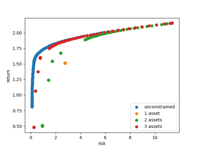
Efficient frontiers for various cardinality constraints

Of course all cardinality constrained portfolios are dominated by the unconstrained ones, but restricting the portfolio to three open positions already yields points very close to the unconstrained efficient frontier. The discontinuity of the constrained frontiers is a consequence of the discrete decision of holding a position or not, preventing a smooth progression from one efficient portfolio to another for varying values of \(\gamma\).

1

Gérard Cornuéjols, Javier Peña, and Reha Tütüncü. Optimization Methods in Finance. Cambridge University Press, 2 edition, 2018. doi:10.1017/9781107297340.