Minimum-Cost Flow

The minimum-cost flow problem routes flow through a graph in the cheapest possible way. It is a fundamental problem in graphs; many other graph problems can be modelled in this form, including shortest path, maximum flow, matching, etc.

The first algorithm to solve this problem, proposed by Dantzig 1 2, was called the network simplex (NS) algorithm. Other methods have been proposed since then, but NS remains one the most efficient approaches. Competitive methods on larger networks include cost-scaling methods (e.g. variants of the push-relabel algorithm by Goldberg and Tarjan3). For a more detailed comparison see, for example, Kovács4.

Problem Specification

For a given graph \(G\) with set of vertices \(V\) and edges \(E\). Each edge \((i,j)\in E\) has the following pair of attributes:

• cost: \(c_{ij}\in \mathbb{R}\);

• capacity: \(B_{ij}\in\mathbb{R}\).

Each vertex \(i\in V\) has a demand \(d_i\in\mathbb{R}\) that can be positive (requesting flow), negative (supplying flow), or zero (a transshipment node).

The problem can be stated as finding the flow with minimal total cost such that:

• the demand at each vertex is met exactly; and

• the flow respects the capacity limit.

Background: Optimization Model

This Mod is implemented by formulating a Linear Program (LP) and solving it using Gurobi. Let us define a set of continuous variables \(x_{ij}\) to represent the amount of non-negative (\(\geq 0\)) flow going through an edge \((i,j)\in E\).

The formulation can be stated as follows:

\[\begin{split}\begin{alignat}{2} \min \quad & \sum_{(i, j) \in E} c_{ij} x_{ij} \\ \mbox{s.t.} \quad & \sum_{j \in \delta^+(i)} x_{ij} - \sum_{j \in \delta^-(i)} x_{ji} = d_i & \forall i \in V \\ & 0 \leq x_{ij} \le B_{ij} & \forall (i, j) \in E \\ \end{alignat}\end{split}\]

Where \(\delta^+(\cdot)\) (\(\delta^-(\cdot)\)) denotes the outgoing (incoming) neighbours.

The objective minimises the total cost over all edges.

The first constraints ensure flow balance for all vertices. That is, for a given node, the incoming flow (sum over all incoming edges to this node) minus the outgoing flow (sum over all outgoing edges from this node) is equal to the demand. Clearly, in the case when the demand is 0, the outgoing flow must be equal to the incoming flow. When the demand is negative, this node can supply flow to the network (outgoing term is larger), and conversely when the demand is negative, this node can request flow from the network (incoming term is larger).

The last constraints ensure non-negativity of the variables and that the capacity limit on each edge is not exceeded.

Code and Inputs

For this Mod, one can use input graphs of different types:

• pandas: using a pd.DataFrame;

• NetworkX: using a nx.DiGraph or nx.Graph;

• SciPy.sparse: using sp.sparray matrices and NumPy’s np.ndarray.

An example of these inputs with their respective requirements is shown below.

scipy.sparsenetworkxpandas

>>> from gurobi_optimods import datasets
>>> G, capacities, cost, demands = datasets.simple_graph_scipy()
>>> G
<5x6 sparse array of type '<class 'numpy.int64'>'
        with 7 stored elements in COOrdinate format>
>>> print(G)
  (0, 1)        1
  (0, 2)        1
  (1, 3)        1
  (2, 3)        1
  (2, 4)        1
  (3, 5)        1
  (4, 5)        1
>>> print(capacities)
  (0, 1)        2
  (0, 2)        2
  (1, 3)        1
  (2, 3)        1
  (2, 4)        2
  (3, 5)        2
  (4, 5)        2
>>> print(cost)
  (0, 1)        9
  (0, 2)        7
  (1, 3)        1
  (2, 3)        10
  (2, 4)        6
  (3, 5)        1
  (4, 5)        1
>>> print(demands)
[-2  0 -1  1  0  2]

Three separate sparse matrices specify the adjacency matrix, the capacity of each edge, and the cost of each edge. A single array specifies the demand at each node.

Solution

Depending on the input of choice, the solution also comes with different formats.

scipy.sparsenetworkxpandas

>>> from gurobi_optimods import datasets
>>> from gurobi_optimods.min_cost_flow import min_cost_flow_scipy
>>> G, capacities, cost, demands = datasets.simple_graph_scipy()
>>> obj, sol = min_cost_flow_scipy(G, capacities, cost, demands, verbose=False)
>>> obj
31.0
>>> sol
<5x6 sparse array of type '<class 'numpy.float64'>'
        with 5 stored elements in COOrdinate format>
>>> print(sol)
  (0, 1)        1.0
  (0, 2)        1.0
  (1, 3)        1.0
  (2, 4)        2.0
  (4, 5)        2.0

The min_cost_flow_scipy function returns the cost of the solution as well as a sp.sparray that provides the amount of flow for each edge in the solution (but only for edges with non-zero flow).

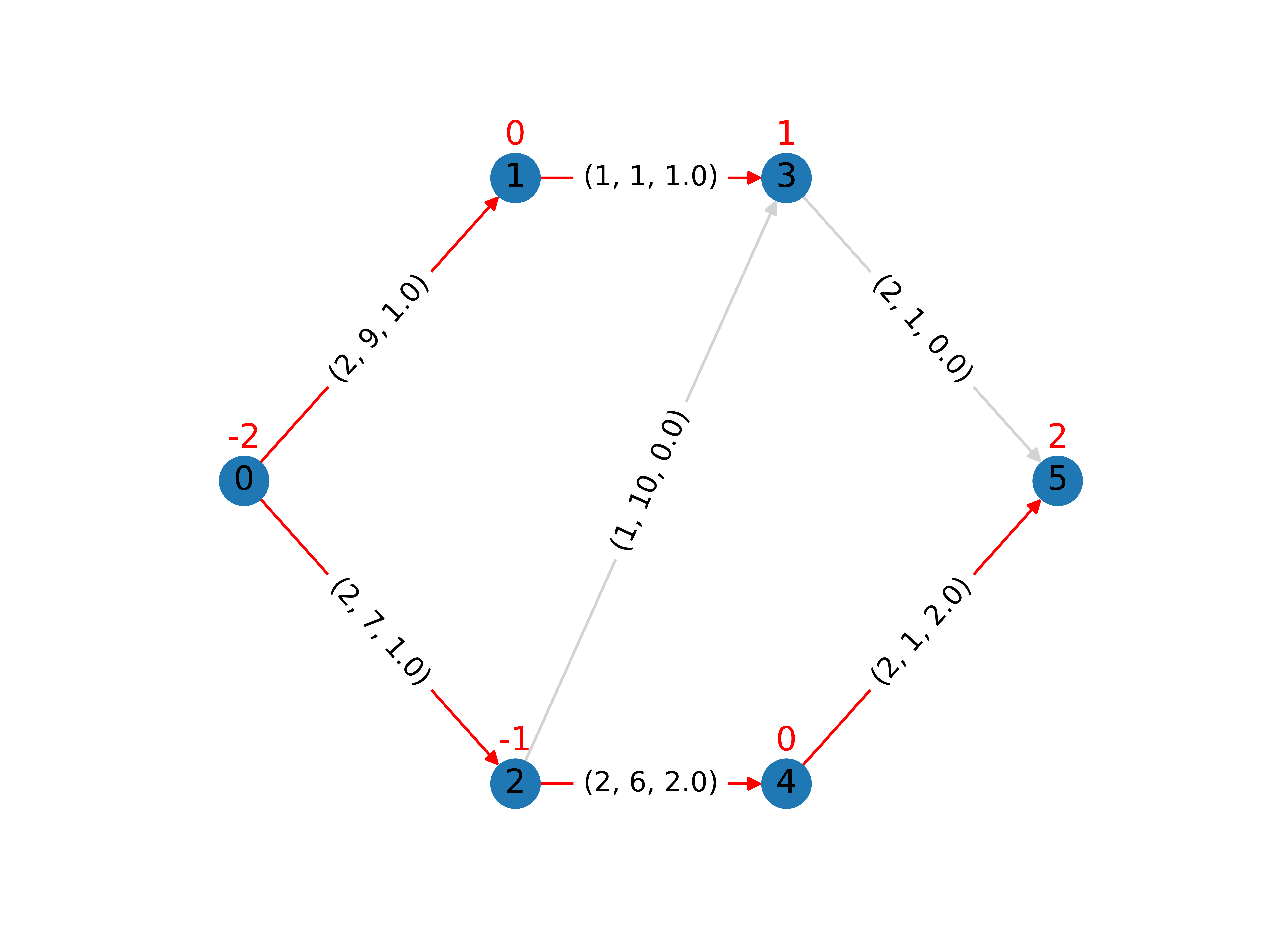
The solution for this example is shown in the figure below. The edge labels denote the edge capacity, cost and resulting flow: \((B_{ij}, c_{ij}, x^*_{ij})\). Edges with non-zero flow are highlighted in red. Also the demand for each vertex is shown on top of the vertex in red.

In all these cases, the model is solved as an LP by Gurobi (typically using the NS algorithm).

1

George B Dantzig. Application of the simplex method to a transportation problem. Activity analysis and production and allocation, 1951.

2

George Dantzig. Linear programming and extensions. Princeton university press, 1963.

3

Andrew V Goldberg and Robert E Tarjan. Finding minimum-cost circulations by successive approximation. Mathematics of Operations Research, 15(3):430–466, 1990.

4

Péter Kovács. Minimum-cost flow algorithms: an experimental evaluation. Optimization Methods and Software, 30(1):94–127, 2015.