Optimal Power Flow
The operation of power systems relies on a number of optimization tasks known as Optimal Power Flow (OPF) problems. The objective of a standard OPF problem is to minimize operational costs such that the underlying grid constraints on generation, demand, and voltage limits are satisfied.
This Mod considers the Alternating Current (AC) and Direct Current (DC) OPF formulations. The ACOPF problem, in its natural form, requires the introduction of complex numbers to formulate voltage constraints. This Mod uses a cartesian-coordinates formulation of ACOPF that reformulates complex-valued terms via nonconvex quadratic relationships. The DCOPF problem approximates the ACOPF problem by making additional assumptions to produce linear constraints. While the additional assumptions result in a potential loss of solution accuracy, they make the DCOPF problem much easier to solve. This is especially useful if the solution accuracy can be neglected in favour of solution time and problem size. Please refer to the Full Problem Specification for full details of the formulations.
Here we assume basic familiarity with concepts such as voltage (potential energy), current (charge flow), and power (instantaneous energy generation or consumption). The engineering community also uses the terms bus to refer to nodes in a network and branch to refer to arcs in a network (a connection between two buses, typically a line or a transformer). Please refer to the Recommended Literature section for more details and comprehensive descriptions of power systems and the underlying problems.
MATPOWER Case Input Format
This Mod has multiple API functions, each of which accepts a dictionary as input
describing an OPF case. This case dictionary follows the MATPOWER Case Format
conventions
and holds all essential information about the underlying network: buses, branch
connections, and generators. Several pre-defined MATPOWER cases can be loaded
directly using the gurobi_optimods.datasets module. The following code loads
an example case with 9 buses and displays the key fields:
baseMVA holds the base units of voltage for this case.
>>> from gurobi_optimods import datasets
>>>
>>> case = datasets.load_opf_example("case9")
>>> case['baseMVA']
100.0
Each entry in the list case['bus'] represents a bus in the network.
>>> from pprint import pprint
>>> from gurobi_optimods import datasets
>>>
>>> case = datasets.load_opf_example("case9")
>>> pprint(case['bus'][0])  # The first bus
{'Bs': 0.0,
 'Gs': 0.0,
 'Pd': 0.0,
 'Qd': 0.0,
 'Va': 0.0,
 'Vm': 1.0,
 'Vmax': 1.1,
 'Vmin': 0.9,
 'area': 1.0,
 'baseKV': 345.0,
 'bus_i': 1,
 'type': 3,
 'zone': 1.0}
Each entry in the list case['branch'] represents a branch in the
network. Note that the fbus and tbus fields must refer to a bus
by its bus_i value.
>>> from pprint import pprint
>>> from gurobi_optimods import datasets
>>>
>>> case = datasets.load_opf_example("case9")
>>> pprint(case['branch'][0])  # The first branch
{'angle': 0.0,
 'angmax': 360.0,
 'angmin': -360.0,
 'b': 0.0,
 'fbus': 1,
 'r': 0.0,
 'rateA': 250.0,
 'rateB': 250.0,
 'rateC': 250.0,
 'ratio': 0.0,
 'status': 1.0,
 'tbus': 4,
 'x': 0.0576}
Each entry in the list case['gen'] represents a generator in the
network. Note that the bus field must refer to a bus by its
bus_i value.
>>> from pprint import pprint
>>> from gurobi_optimods import datasets
>>>
>>> case = datasets.load_opf_example("case9")
>>> pprint(case['gen'][0])  # The first generator
{'Pc1': 0,
 'Pc2': 0,
 'Pg': 0,
 'Pmax': 250,
 'Pmin': 10,
 'Qc1max': 0,
 'Qc1min': 0,
 'Qc2max': 0,
 'Qc2min': 0,
 'Qg': 0,
 'Qmax': 300,
 'Qmin': -300,
 'Vg': 1,
 'apf': 0,
 'bus': 1,
 'mBase': 100,
 'ramp_10': 0,
 'ramp_30': 0,
 'ramp_agc': 0,
 'ramp_q': 0,
 'status': 1}
Each entry in the list case['gencost'] corresponds to the generator
at the same position in case['gen'], and defines the cost function
of that generator.
>>> from pprint import pprint
>>> from gurobi_optimods import datasets
>>>
>>> case = datasets.load_opf_example("case9")
>>> pprint(case['gencost'][0])  # Cost function for the first generator
{'costtype': 2.0,
 'costvector': [0.11, 5.0, 150.0],
 'n': 3.0,
 'shutdown': 0.0,
 'startup': 1500.0}
Warning
The Mod only supports generator costs with costtype = 2 and n
<= 3 (i.e. linear and quadratic cost functions) in the gencost
structure, as these are the most commonly used settings in practice.
If a different costtype or larger value of n value is provided,
an error will be issued.
Cases can also be read directly from MATPOWER format using
read_case_matpower(). This function reads a standard
MATLAB .mat data file holding the case data into the native Python format
accepted by the Mod. For example:
case = opf.read_case_matpower("my_case.mat")
Solving an OPF Problem
After reading in or otherwise generating a MATPOWER case in the format described
above, we can solve an OPF problem defined by the given network data. For this
task, we use the solve_opf() function. We can define
the type of the OPF problem that we want to solve by defining the opftype
argument when calling the function. Currently, the available options are AC,
ACrelax, and DC.
The
ACsetting solves an ACOPF problem defined by the given network data. The ACOPF problem is formulated as a nonconvex bilinear model as described in the ACOPF section of the Full Problem Specification. This setting yields the most accurate model of the physical power system. However, it is also the most difficult problem to solve and thus usually leads to the longer runtimes.The
ACrelaxsetting solves a Second Order Cone (SOC) relaxation of the nonconvex bilinear ACOPF problem formulation defined by the given network data. The relaxation is constructed by dropping nonconvex bilinear terms but simultaneously keeping the convex JABR inequalities, see JABR Relaxation for more details. This setting often yields a good approximation of the physical power system and is of moderate difficulty.The
DCsetting solves a DCOPF problem defined by the given network data. The DCOPF problem is a linear approximation of the ACOPF problem, see DCOPF section of the Full Problem Specification for more details. This setting only yields a crude approximation of the physical power system, but is usually an easy problem that can be solved very quickly even for large networks.
The solve_opf function solves an AC problem unless the opftype
argument specifies otherwise.
from gurobi_optimods import opf
from gurobi_optimods import datasets

case = datasets.load_opf_example("case9")
result = opf.solve_opf(case, opftype="AC")
...
Optimize a model with 73 rows, 107 columns and 208 nonzeros
...
Optimal solution found...
...
Objective value = 5296...
...
ACOPF and Branch Switching models are most often very hard to solve to
optimality. For this reason, it is recommended to specify a solver time limit
using the time_limit parameter. If the problem has not been solved to
optimality within the time limit, the best known solution will be returned.
result = opf.solve_opf(case, opftype="AC", time_limit=60)
Solution Format
The Mod returns the result as a dictionary, following the same MATPOWER Case Format conventions as the case dictionary. However, in the result dictionary some object entries are modified compared to the input case dictionary. These modified fields hold the solution values of the optimization. There are also additional fields to store the solution information, as specified below.
The bus entries result['bus'][i]['Vm'] and
result['bus'][i]['Va'] store the voltage magnitude (Vm) and voltage
angle (Va) values in the OPF solution for bus i.
If a DCOPF problem was solved, additional fields
result['bus'][i]['mu'] hold the shadow prices for balance
constraints at bus i.
>>> result['bus'][0]
{... 'Vm': 1.09..., 'Va': 0, ...}
The additional branch entries populated in the solution data are:
Pf: real power injection at the “from” end of the branch,Pt: real power injection at the “to” end of the branch,Qf: reactive power injection at the “from” end of the branch, andQt: reactive power injection at the “to” end of the branch.
The switching field defines whether a branch is turned on (1) or off
(0) in the given result.
>>> result['branch'][1]
{... 'Pf': 35.2..., 'Pt': -35.0..., 'Qf': -3.8..., 'Qt': -13.8..., ...}
Then gen entries result['gen'][i]['Pg'] and
result['gen'][i]['Qg'] hold the real and reactive power injection
values, respectively, for the \(i^{th}\) generator.
>>> result['gen'][2]
{... 'Pg': 94.1..., 'Qg': -22.6..., ...}
Plotting Feasible Solutions
In addition to solving an OPF problem, this Mod also provides plotting functions to display graphical representation of the network and the OPF result. There are already very involved graphical tools to represent OPF solutions provided by other packages such as:
thus the graphical representation provided by this Mod is kept intentionally
simple. In order to use this functionality, it is necessary to install the
plotly package as follows:
pip install plotly
In order to plot a previously obtained result, you must provide \((x, y)\) coordinates for all buses in the network. Coordinates are provided as a dictionary mapping bus IDs to coordinates. The OptiMods datasets module provides an example set of coordinates for plotting the 9 bus test case:
>>> coordinates = datasets.load_opf_extra("case9-coordinates")
>>> from pprint import pprint
>>> pprint(coordinates)
{1: (44.492, -73.208),
 2: (41.271, -73.953),
 3: (41.574, -73.966),
 4: (40.814, -72.94),
 5: (43.495, -76.451),
 6: (42.779, -78.427),
 7: (44.713, -73.456),
 8: (43.066, -76.214),
 9: (43.048, -78.854)}
Given a solution and a coordinate mapping, the plotting functions return plotly figures which can be displayed in a web browser. In the following code, we solve the DCOPF problem for a real-world dataset for the city of New York and produce a solution plot:
case = datasets.load_opf_example("caseNY")
solution = opf.solve_opf(case, opftype='DC')
coordinates = datasets.load_opf_extra("caseNY-coordinates")
fig = opf.solution_plot(case, coordinates, solution)
fig.show()  # open plot in a browser window
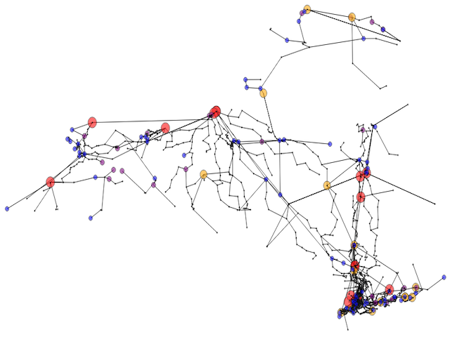
DCOPF solution for the New York power grid example dataset
The above image shows the grid solution generated from the given network data, plotted using the provided coordinates. The colored circles depict generators and the amount of power they generate:
Black bus: Power generation \(\leq 75\) and load \(< 50\)
Blue bus: Power generation \(\leq 75\) and load \(\geq 50\)
Purple bus: Power generation \(> 75\)
Orange bus: Power generation \(> 150\)
Red bus: Power generation \(> 500\)
Branch Switching
An important extension of the OPF problem is Branch Switching, where branches may be turned off. Note that already turning off a single branch changes the whole power flow through the network. Thus in practice, it is rare that branches are turned off at all, even if this option is enabled. If any are turned off, then it is usually only a small fraction of the overall power grid. For the mathematical formulation, please refer to the Branch Switching subsection of the Full Problem Specification.
To enable branch switching in a given OPF problem, set the branch_switching
argument to True when calling gurobi_optimods.opf.solve_opf(). The Mod
additionally offers the possibility to control the number of branches that must
remain switched on via the min_active_branches argument. In practice, it is
expected that only a very small fraction of branches are turned off. Thus, the
default value of the min_active_branches argument is 0.9 (90%). In the
following example, we solve a modified version of the 9 bus network to see
whether branch switching allows a better solution.
case = datasets.load_opf_example("case9-switching")
result = opf.solve_opf(
    case, opftype="AC", branch_switching=True, min_active_branches=0.1
)
Plotting the resulting solution shows that one branch has been turned off in the optimal solution. Please note, that the used examplary network has been artificially adjusted to achieve this result and this is not the usual behavior in a realistic power grid of such small size.
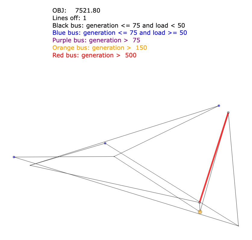
Branch switching solution. The plot highlighted the switched-off branch in red
Violations for Pre-defined Voltage Values
In practice we may have voltage magnitudes and voltage angles for each bus at
hand and would like to know whether these values are actually feasible within a
given network. To tackle this problem, we can use the
gurobi_optimods.opf.compute_violations() function. This function takes a
set of bus voltages in addition to the case data and returns the computed
violations in this voltage solution.
Bus voltages are provided as a dictionary mapping the Bus ID to a pair \((V_m, V_a)\) where \(V_m\) is the voltage magnitude and \(V_a\) is the voltage angle. An example is provided for the 9 bus case:
>>> voltages = datasets.load_opf_extra("case9-voltages")
>>> pprint(voltages)
{1: (1.089026, 0.0),
 2: (1.099999, 20.552543),
 3: (1.090717, 16.594399),
 4: (1.084884, -2.408447),
 5: (1.096711, 2.43001),
 6: (1.099999, 11.859651),
 7: (1.072964, 9.257936),
 8: (1.066651, 11.200108),
 9: (1.08914, 2.847507)}
Using this voltage data, we can check for possible model violations by calling
the gurobi_optimods.opf.compute_violations() function. The function
returns a dictionary which follows the MATPOWER Case Format with
additional fields storing the violations for particular buses and branches.
The following fields in the violations dictionary are added to store violations data:
violation['bus'][i]['Vmviol']Voltage magnitude violation at bus iviolation['bus'][i]['Pviol']real power injection violation at bus iviolation['bus'][i]['Qviol']reactive power injection violation at bus iviolation['branch'][i]['limitviol']branch limit violation at branch i
volts_dict = datasets.load_opf_extra("case9-voltages")
case = datasets.load_opf_example("case9")
violations = opf.compute_violations(case, volts_dict)
>>> print(violations['branch'][6]['limitviol'])
66.33435016796234
>>> print(violations['bus'][3]['Pviol'])
-318.8997836192236
In this case, the limit at branch 6 and the real power injection at bus 3 are violated by the given input voltages.
Plotting Violations
Similar to generating a graphical representation of a feasible solution, it is
also possible to generate a figure representing the violations within a given
power grid. We can use the gurobi_optimods.opf.violation_plot() for this.
The violations result is provided as input, along with the case and coordinate
data, to produce this plot.
voltages = datasets.load_opf_extra("case9-voltages")
case = datasets.load_opf_example("case9")
coordinates = datasets.load_opf_extra("case9-coordinates")
violations = opf.compute_violations(case, voltages)
fig = opf.violation_plot(case, coordinates, violations)
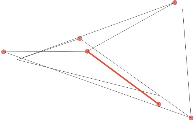
The above image shows the power grid generated from the given network data together with coordinate and violation data. The red circles depict buses where the voltage magnitude or real or reactive power injections are violated. Red marked branches depict branches with violated limits.
Recommended Literature
Power systems and the optimal power flow problem are well studied. For a more comprehensive descrition, we recommend the following literature.
G. Andersson. Modelling and Analysis of Electric Power Systems. Power Systems Laboratory, ETH Zürich, 2004.
A.R. Bergen and V. Vittal. Power Systems Analysis. Prentice-Hall, 1999.
D. Bienstock. Electrical Transmission Systems Cascades and Vulnerability, an Operations Research viewpoint. SIAM, 2015. ISBN 978-1-61197-415-7.
D.K. Molzahn and I.A. Hiskens. A survey of relaxations and approximations of the power flow equations. Foundations and Trends in Electric Energy Systems, 4:1–221, 2019.
J.D. Glover, M.S. Sarma, and T.J. Overbye. Power System Analysis and Design. CENGAGE Learning, 2012.
Formulation Details
Full details of the formulations used in the OPF Mod are given in the following sections: